

V4r4 User Guide
Documentation Files
| Name | Description |
|---|---|
| README | File containing information |
| v4r4_synopsis.pdf | Synopsis of V4r4 estimation |
| v4r4_user_guide.pdf | User guide (PDF format) |
| v4r4_overview_plots.pdf | Plots of V4r4 |
| ECCO_V4r4_reproduction_howto.pdf | Reproducing V4r4 results with MITgcm |
| available_diagnostics.log | A full list of available diagnostics with a short description (for a slightly more detailed description of diagnostics, check out the readme file*) |
| costfunction0059 | Costs with the grid size factor (gamma, Cf. v4r3_summary.pdf [Section 4.3] for an explanation of gamma) |
| STDOUT.0000 | Model standard output |
1. Introduction
This note describes the directory structure and content of ECCO Version 4, Release 4's (V4r4) data server. Covering the time period from 1992 through 2017, ECCO V4r4 synthesizes a general circulation model (MITgcm) and most of available satellite and in situ data to produce a physically consistent ocean estimate of which property budgets can be closed. The data that are used to constrain the model include satellite altimetry (sea surface height, SSH), GRACE ocean bottom pressure (OBP), AVHRR sea surface temperature (SST), Aquarius sea surface salinity (SSS), Argo, CTD, XBT, ITP, APB, Glider, TAO mooring temperature and salinity data, sea-ice measurements, and global mean SSH and OBP. The estimate uses the adjoint method to iteratively minimize the squared sum of weighted model-data misfits and control adjustments. A more detailed summary of the estimate can be found in Fukumori et al. (2019).
This document is an update of the overview document of ECCO Version 4, Release 3's (V4r3) (Wang et al., 2017). A few updates are as follows. In Section 3, the document describes the new data server, ECCO Drive, that has replaced the anonymous ftp server used for V4r3. Fields that are not presented in V4r3, as a result of the atmospheric pressure forcing introduced in V4r4, are discussed in Section 4.4.1. V4r4 has a complete set of daily mean and instantaneous fields, as opposed to V4r3's handful daily fields, which are described in Section 4.6. Finally, we describe a flux-forced configuration of V4r4 that is included as part of the product (Section 6).
2. Model

The model that is used to produce V4r4 is MITgcm version checkpoint66g. Wang (2019) gives a detailed description about how to download the code, data, and any needed auxiliary files to reproduce V4r4.
The grid used in V4r4 is the so-called LLC90 (Lat-Lon-Cap 90) grid (Fig. 1a) that has five faces covering the whole globe, with simple latitude-longitude grid between 70°S and 57°N and an Arctic cap (Forget et al., 2015). The dimensions for the five faces are [90x270], [90x270], [90x90], [270x90], and [270x90] where each face consists of tiles dimensioned 90x90 (thus LLC90) (Figs. 1a & 1b). The horizontal resolution varies spatially from 22km to 110km, with the highest resolution in high latitudes and lowest resolution in mid latitudes. The deepest ocean bottom is set to 6145m below the surface, with the vertical grid spacing increasing from 10m near the surface to 457m near the ocean bottom.
3. Data Server
The ECCO data server is a Web Distributed Authoring and Versioning (WebDAV) server, called ECCO Drive. In order to access the ECCO products, ECCO Drive requires each user first register for a NASA Earthdata account. ECCO Drive offers a familiar http-like interface for users to browse and download data through their browser. More importantly, it allows scripted data extracting via a command line interface, e.g. using wget to download the data. Users can also mount ECCO Drive as a network disk. The help page lists various methods accessing the products. Users can also find more details about various options to download the files on the ECCO V4r4's webpage.
ECCO Drive automatically assigns each user a WebDAV password that one could find in https://ecco.jpl.nasa.gov/drive/ (middle text box). The WebDAV password is different from the password for one's Earthdata account. Users need to enter the WebDAV password, not the Earthdata account password, to use wget or mount ECCO Drive to their local machines.
A sample wget command to download V4r4's monthly potential temperature fields on the native grid is as follows:
wget -r --no-parent --user YOUREARTHDATAUSERNAME --ask-password https://ecco.jpl.nasa.gov/drive/files/Version4/Release4/nctiles_monthly/THETA
When prompted for password, you need to enter your ECCO Drive's WebDAV password, not your Earthdata account's password.
Due to NASA's mandate to disallow the use of the ftp protocol for data access, the ECCO anonymous ftp server at https://ecco.jpl.nasa.gov/drive/files is no longer available.
4. Directory Structure
In this section, we describe the directory structure of V4r4's data server. Each subdirectory has a short README file that lists all the sub-directories and files in that directory along with a brief description. The directory structure is similar to that of Release 3's (Wang et al., 2017).
4.1 Documentation
The directory doc contains a few useful documents that include an overview of V4r4's directory and file structures, a summary of V4r4 (Fukumori et al., 2020), a note about how to reproduce V4r4 results, a set of analysis plots generated using gcmfaces (see Section 7, Software), and a note on analyzing budgets (Piecuch, 2022). Also included are summary files of all cost functions (costfunction*) and a "standard output file" (STDOUT.0000) that the model creates during its integration with information about the model configuration and useful measures of the model state.
4.2 Model Grid
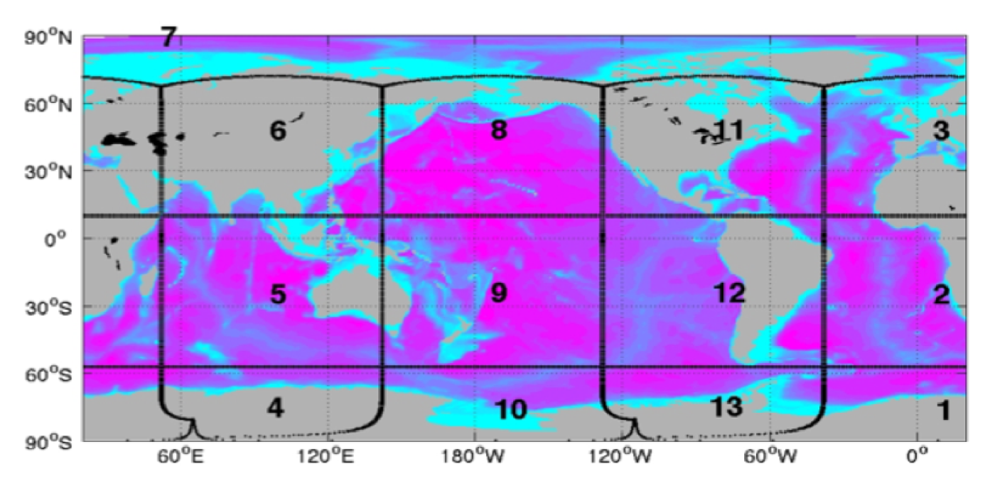
The model grid information can be found in the subdirectory nctiles_grid. The globe is split into 13 regional tiles (Fig. 2, courtesy of Gaël Forget), with variables that are saved in separate individual files in netCDF format (ECCO-GRID_00.nc to ECCO-GRID_00.nc). Also provided is a single netCDF file of the grid information in ECCO-GRID.nc. These netCDF files can be read by using various netCDF tools from different programming languages and platforms, such as Python, MATLAB, and FORTRAN. Two useful toolboxes, ECCOv4-py and gcmfaces that use Python and MATLAB respectively, have been developed to facilitate the processing of ECCO files. See more details in Section 7 (Software).
4.3 Introduction to Fields
V4r4 provides the model state and forcing on either model native grid or regular 0.5o by 0.5o lat-lon grid. Complete daily and monthly fields are provided, including averages and instantaneous fields that allow one to close property budgets on either a daily or monthly basis. The complete daily fields are an improvement from V4r3 to make it possible to study higher frequency processes (e.g. mixed-layer dynamics). In addition to daily and monthly fields, V4r4 has some auxiliary variables in hourly resolution, including the core products of International Earth Rotation Services (IERS) Special Bureau for the Oceans. These SBO core products include global ocean mass, center of mass, and ocean angular momentum.
4.4 Monthly Average Model Fields
The nominal model output is its monthly fields (nctiles_monthly). Each subdirectory inside nctiles_monthly contains netCDF files for a particular variable, as indicated by the name of the subdirectory. The files of each variable are organized by year (subdirectory) and each yearly field is split 12 monthly netCDF files. Each file contains the complete global field with all 13 tiles. Some of the most commonly used fields, like velocity components, potential temperature, salinity, SSH, and OBP are UVEL, VVEL, THETA, SALT, SSHDYN, and and OBPNOPAB. The two fields, SSHDYN and OBPNOPAB, are the equivalents of ECCO v3r3's SSH and OBP. The new names reflect the fact that ECCO V4r4 has the additional air pressure forcing to the forcing used in V4r3, and therefore have to be corrected to generate equivalent fields to V4r3's SSH and OBP. SSHDYN is the sea surface height corrected with the inverse barometer correction, and OBPNOPAB is the same as OBP, but with the global ocean mean of air pressure removed. More details are included in the following section (Corrected Sea Level and Ocean Bottom Pressure).
The netCDF files can be read by ECCOv4-py or gcmfaces, the two toolboxes developed using Python and MATLAB for processing ECCO V4 files. See more details in Section 7 (Software).
4.4.1 Corrected Sea Level and Ocean Bottom Pressure
ECCO V4r4 is forced with high-frequency atmosphere pressure, although the air pressure is not part of the control variables. The atmosphere pressure is from ERA-Interim, filtered with a 3-year running mean to remove the air tide (Michael Schindelegger, personal communication, 2019). In contrast, V4r3 was not forced with air pressure. The added air pressure forcing makes high-frequency ocean bottom pressure closer to gauge measurements (Ponte et al., 2019).
There are three variables, ETAN, SSHDYN, and SSH, describing sea surface height. ETAN is the height of the model's liquid ocean surface, whereas SSHDYN and SSH are the corrected sea surface height. SSHDYN is commonly called the dynamic sea surface height, calculated by correcting model sea level anomaly ETAN for three effects : a) spurious mass fluxes incurred by density changes in the Boussinesq volume-conserving model (Greatbatch correction, Griffies and Greatbatch, 2012), b) the inverted barometer (IB) effect (see SSHIB) and c) upward sea level displacement due to submerged sea-ice and snow (see sIceLoad). SSHDYN can be compared with the variable "SSH" in previous ECCO products that did not include atmospheric pressure loading (e.g., Version 4 Release 3). SSH is the same as SSHDYN, but is NOT corrected for the IB effect. All three variables of sea surface height reflect mass changes caused by freshwater input. Since the altimetry measurement is normally corrected with IB effect, variable SSHDYN, not SSH or ETAN, provides the model equivalent of IB-corrected altimetry sea level measurements. Use SSH for comparisons with altimetry data products that do NOT apply the IB correction.
Similarly, there are three variables, PHIBOT, OBPNOPAB, and OBP for ocean bottom pressure. PHIBOT is model ocean bottom pressure (in m2s-2) that generally cannot be compared with data and accounts for the time-varying change of grid cell thicknesses allowed by the z* coordinate system. OBPNOPAB is model ocean bottom pressure in equivalent sea level in meters, calculated by dividing PHIBOT by gravity (9.81 m s-2), and correcting for a) spurious mass fluxes incurred by density changes in the Boussinesq volume-conserving model (Greatbatch correction; see above) and b) spatial mean atmospheric pressure variations over the global ocean. OBPNOPAB can be compared with the variable OBP in previous ECCO products that did not include atmospheric pressure loading (e.g., Version 4 Release 3). OBP in the current product (V4r4) is the same as OBPNOPAB, but includes the spatial mean atmospheric pressure variations over the global ocean. Use OBPNOPAB for comparisons with ocean bottom pressure data products that have been corrected for global mean atmospheric pressure variations. GRACE data typically ARE corrected for global mean atmospheric pressure variations. In contrast, ocean bottom pressure gauge data typically ARE NOT corrected for global mean atmospheric pressure variations, and therefore should be compared against OBP.
4.4.2 Native and Geographical Velocity Components
Users are advised to be aware of the directional convention used in the model especially when analyzing the vector fields of the model. Figure 1b illustrates the directional convention used in the LLC grid. Within each face (tile), the x- and y-directions point left-to-right and bottom-to-top in the figure, respectively. As such, in faces 4 and 5, the x- and y-directions point to the south and to the east, respectively. In face 3, the x-direction points to the Pacific Ocean away from the Atlantic, whereas y-direction points to North America away from Asia. For user convenience, conventional eastward and northward velocity components (EVEL and NVEL) are provided as diagnostic output, in addition to that in the model's native direction (UVEL and VVEL) (see Table 1).
| Filename | Description |
|---|---|
| UVEL | X-component of velocity (m/s). |
| VVEL | Y-component of velocity (m/s). |
| EVEL | Zonal component of velocity (m/s). Positive is eastward. |
| NVEL | Meridional component of velocity (m/s). Positive is northward. |
4.4.3 Advective and Diffusive Fluxes
The files with their names starting with "ADV" and "DF" indicate advective and diffusive fluxes, respectively. Similar to velocity, the horizontal components of the native fluxes also follow the model's directional convention. For instance, DFxE_TH means diffusive flux ("DF"), in the model's x-direction ("x"), evaluated explicitly ("E") for potential temperature ("TH"). Table 2 lists all the flux terms for potential temperature. See Piecuch (2022) for how to make use of the flux terms along with forcing terms to close budgets.
| Filename | Description |
|---|---|
| ADVx_TH | X-component ("x") of ADVective flux of potential temperature ("TH") (C m3/s) at a particular grid (i,j,k). Positive to increase temperature at (i,j,k). |
| ADVy_TH | Y-component ("y") of ADVective flux of potential temperature (C m3/s). |
| ADVr_TH | Z-component ("r") of ADVective flux of potential temperature (C m3/s). |
| DFxE_TH | X-component of DiFfusive flux of potential temperature (C m3/s). Explicit part ("E"). |
| DFyE_TH | Y-component of DiFfusive flux of potential temperature (C m3/s). Explicit part. |
| DFrE_TH | Z-component of DiFfusive flux of potential temperature (C m3/s). Explicit part. |
| DFrI_TH | Z-component of DiFfusive flux of potential temperature (C m3/s). Implicit part ("I"). |
4.5 Instantaneous Monthly Model Fields
Besides monthly averages, V4r4 also provides monthly snapshots in the subdirectory nctiles_monthly_snapshots for THETA, SALT, and ETAN. The main purpose of these snapshots is to facilitate budget calculations (see Section 5, Budget Calculation); specifically, monthly mean fluxes that are provided equal changes between these snapshots (as opposed to changes between monthly average states of Section 4.4).
4.6 Daily Model Fields
V4r4 provides a complete set of daily average fields, including ocean state, forcing, and budget terms. This is a big improvement to the nominal monthly fields that V4r3 provided, as now users can close daily property budgets. Because of the large volume of daily fields, the complete set of daily fields are available at NASA's Advanced Supercomputing Division (NAS) data portal. See Table 3 for the directory structure.
| Directory Name | Description |
|---|---|
| nctiles_daily | Daily average fields. |
| nctiles_daily_snapshots | Daily snapshots. |
A subset of daily averages are also available on ECCO Drive for select variables in directory nctiles_daily (Table 4). These daily fields are the mostly commonly used ocean and sea-ice states.
| Directory Name | Description |
|---|---|
| SSHDYN | Dynamic sea surface height anomaly (m) calculated by correcting model level anomaly ETAN for three effects: a) Greatbatch correction, b) the inverted barometer (IB) effect, and c) upward sea level displacement due to submerged sea-ice and snow. See Section 4.4.1. |
| OBPNOPAB | OBPNOPAB (m) is model ocean bottom pressure in equivalent sea level in meters, calculated by dividing PHIBOT by gravity (9.81 m s-2), and correcting for a) Greatbatch correction and b) spatial mean atmospheric pressure variations over the global ocean. See Section 4.4.1. |
| THETA | Ocean potential temperature (°C). |
| SALT | Salinity (psu). |
| SIarea | Fractional sea-ice covered area (m2/m2) |
| SIheff | Effective sea-ice thickness (m) that is defined as actual sea-ice thickness scaled by fractional sea-ice area (SIarea). |
| SIhsnow | Effective snow thickness (m). |
| sIceLoad | Sea-ice and snow loading defined as mass of sea-ice & snow over area (kg/m2). |
| SSH | Sea surface height (m) that is the same as SSHDYN but is not corrected for IB effect. |
| SSHIB | The inverted barometer (IB) correction to model sea level anomaly (ETAN) required to account for sea surface displacement by atmosphere pressure loading. |
| OBP | Ocean bottom pressure (m) that is the same as OBPNOPAB, but includes the spatial mean atmospheric pressure variations over the global ocean. |
4.7 Data Used to Constrain the Model
The subdirectory input_ecco includes the data used to constrain the model (Table 5). Most of the files are in binary format on the native model grid. Each 2-d field is of size 90x1170. The files are provided as binary files, not in netCDF format, as the files in binary format are needed to reproduce V4r4's results. A sample MATLAB script that reads and displays a 2-d binary field on the model grid is presented in Software, Box 1.
| Directory Name | Description |
|---|---|
| input_sla | Daily RADS altimetry SSH data (m). |
| input_bp | Monthly GRACE ocean bottom pressure (OBP) from JPL RL05 mascon solutions (cm). |
| input_insitu | In situ profile data. |
| input_sst | Reynolds daily SST (°C). |
| input_sss | Aquarius monthly SSS (psu). |
| input_nsidc | Daily sea-ice concentration from NSDIC (unitless). |
| input_other | Climatology TS from WOA'09, mean dynamic topography (DTU17MDT) from DTU Space, global mean SSH & OBP etc. See README there. |
4.8 Model Equivalent of In-situ Data
The model equivalents of the in situ data in netCDF format are in profiles. The model fields are sampled on the fly at the time and location of the in situ data to generate the model equivalents. For each in situ file in input_ecco/input_insitu, there is a corresponding file of the model equivalent in profiles.
4.9 Interpolated Monthly Fields
Since V4 grid is not a regular lat-lon grid, we have also provided interpolated monthly averages on a regular 0.5° by 0.5° grid in interp_monthly for user convenience. However, note that the interpolated fields should not be used for budget calculations, as the interpolation does not preserve integrated quantities. The fields on the native V4 grid should be used instead. The interpolated files are in netCDF format, with one file for one particular variable.
4.10 Atmospheric Forcing
In addition to all atmospheric forcing used in V4r3, V4r4 has the ERA-Interim surface atmospheric pressure forcing. The atmospheric forcing files are in the subdirectory input_forcing. The directory contains binary yearly files of 6-hourly forcing on V4 grid (Table 6). All forcing fields except for wind speed (eccov4r4_wspeed_YYYY) and air-pressure (eccov4r4_pres_YYYY) are the sum of ERA-Interim forcing and the corresponding control adjustment that has been estimated. Wind speed is not a control variable and is only ERA-Interim wind speed interpolated onto the V4 grid. Air-pressure is also not part of the control variables, and is a filtered version of ERA-Interim 6-hourly surface atmospheric press forcing. The original ERA-Interim pressure is filtered by Michael Schindelegger (U. Bonn) to remove air tides that are not well resolved in the 6-hourly forcing (cf. Fukumori, et al. 2019).
| Filename (replace YYYY with year) | Description |
|---|---|
| eccov4r4_dlw_YYYY | Yearly files for 6-hourly downward longwave (W/m2) in binary format. Positive to decrease ocean temperature. |
| eccov4r4_dsw_YYYY | Downward shortwave (W/m2). Positive to decrease ocean temperature. |
| eccov4r4_rain_YYYY | Precipitation (m/s). Positive to increase sea level. |
| eccov4r4_spfh2m_YYYY | Specific humidity at 2m above the sea surface. |
| eccov4r4_tmp2m_YYYY | Air temperature at 2m above the sea surface. |
| eccov4r4_ustr_YYYY | East-West component of wind stress (N/m2). Positive from east to west. |
| eccov4r4_vstr_YYYY | North-South component of wind stress (N/m2). Positive from north to south. |
| eccov4r4_wspeed_YYYY | Wind speed at 10m above ocean surface (m/s). |
| eccov4r4_pres_YYYY | Air-pressure (N/m2) at sea-level. It is a filtered version of ERA-Interim surface pressure, interpolated to V4 grid. |
4.11 Input Files
The subdirectory input_init includes other files that are needed to reproduce V4r4 (Table 7).
| Directory / File Name | Description |
|---|---|
| NAMELIST | Namelist such as file "data", "data.ctrl", etc. |
| error_weight | Data error (data_error) and control weight (ctrl_weight). |
| bathy_eccollc_90x50_min2pts.bin | Bathymetry (m). |
| pickup* files | Initial condition. |
| xx* files | Control adjustments on V4 grid. |
| total_diffkr*, total_kap* | Mixing coefficients. |
| tile* files | Grid files needed to run the model. |
| smooth* files | Smoothing operator related files. |
| fenty_biharmonic_visc_v11.bin | Bi-harmonic coefficients (m4/s). |
| runoff-2d-Fekete-1deg-mon-V4-SMOOTH.bin | Climatology river runoff (m/s). Positive to increase sea level. |
| geothermalFlux.bin | Time-invariant geothermal flux (W/m2). Positive to increase ocean temperature. |
4.12 Other Fields
V4r4 has some auxiliary fields in the subdirectory other (Table 8). These files include the binary yearly files of 6-hourly unadjusted atmospheric forcing (interpolated ERA-interim forcings on V4 grid). By taking the difference between the total atmospheric forcing and the unadjusted forcing one could obtain the dimensional atmospheric control adjustments. File "SBO_global.nc" contains hourly core products for Earth rotation of the International Earth Rotation and Reference Systems Service (IERS), including contributions of ocean mass, oceanic angular momentum, and the ocean's center-of-mass.
| Directory / File Name | Description |
|---|---|
| input_forcing_unadjusted | Unadjusted atmospheric forcings on V4 grid. |
| adjustments | Dimensional control adjustments for control variables other than atmospheric control variables. |
| SBO_global.nc | IERS Special Bureau for the Oceans (SBO) core products for Earth rotation. |
| Pa_global.nc | The hourly spatial mean of air pressure averaged over the global ocean. |
5. Budget Calculation
Monthly mean fluxes are provided in directory nctiles_monthly. Piecuch (2022) provides a practical note on how to analyze budgets using these fields, describing the calculation both in pseudo code and in MATLAB (gcmfaces library; see Section 7 (Software). Although the note was written for V4r3, the budget can be calculated similarly for V4r4.
6. Flux-forced Configuration for V4r4
A flux-forced configuration of V4r4 is provided as part of release 4. This configuration can produce the same forward results as V4r4's, but differs from V4r4 by reading the atmospheric fluxes from pre-computed files. In contrast, V4r4 uses the bulk-formula to compute the air-sea fluxes as well as the ice-ocean and ice-atmosphere fluxes. The fluxes would change along with underling ocean and/ice states. However, sometimes one would want to separate contributions of various fluxes to a particular ocean quantity and need to have the fluxes independent upon the underlining ocean states. The flux-forced configuration provides such capability, since the fluxes are pre-computed. Potential usage includes forward sensitivity experiments, adjoint reconstruction, and others.
The code and namelists are on GitHub. The forcing and other input files of large sizes are in directory other/flux-forced. A user would follow the similar steps described in the V4r4 reproduction document (Wang, 2019), but use the updated code and namelists from GitHub and forcing and other input files from other/flux-forced.
7. Software
ECCOv4-py is a Python library that can be used to analyze ECCO Version 4 state estimate, including V4r4. It includes tools for loading, plotting, and processing the fields. An example of its usage is that almost all of the netCDF files for V4r4 in the data server were generated using ECCOv4-py.
The package is available on GitHub. A detailed tutorial about how to use V4r4 with ECCOv4-py can be found on the readthedocs page, including installation instructions.
Gaël Forget from MIT has created a MATLAB/Octave toolbox called gcmfaces (Forget 2017) to facilitate analysis of gridded earth variables on different grids, including the llc90 grid used in V4r4. The gcmfaces user guide provides a brief description about gcmfaces, including the URLs of the code repositories on GitHub and the documentation pages on readthedocs. The current code repository of gcmfaces is on GitHub, with the documentation on its readthedocs page. The gcmfaces toolbox includes a tutorial script called gcmfaces_demo.m that illustrates how to make use of gcmfaces. A companion MATLAB/Octave toolbox called MITprof to process and analyze in situ profile data is also available on GitHub.
Assume that one has downloaded V4r4 products and successfully installed gcmfaces and all necessary data files according to Section 1 of the gcmfaces' user guide. Provided below are a couple of sample MATLAB scripts in the context of gcmfaces to read and display the binary and netCDF files of V4r4.
p = genpath('gcmfaces/'); addpath(p);
p = genpath('m_map/'); addpath(p);
%Load the grid.
grid_load;
% Define global variables
gcmfaces_global;
%Type in the path of the grid directory of V4r4 that one has downloaded from
% https://ecco.jpl.nasa.gov/drive/files/Version4/Release4/nctiles_grid/
% e.g. '/mydir/v4r4/nctiles_grid/';
%Read in binary files
%To read in and display the 15th 6-hourly record of the E-W wind stress for year 1992
%Read in data
dirv4r4 = '/mydir/v4r4/';
ff= [dirv4r4 'input_forcing/' 'eccov4r4_ustr_1992'];
fld = read_bin(ff,15,0); %read in the 15th 2-D record
%Display
figure;
[X,Y,FLD]=convert2pcol(mygrid.XC,mygrid.YC,fld); pcolor(X,Y,FLD);
if ~isempty(find(X>359)); axis([0 360 -90 90]); else; axis([-180 180 -90 90]); end;
dd1 = 1;
cc=[-1:0.1:1]*dd1; % color bar set to -1 to 1 N/m2
shading flat; cb=gcmfaces_cmap_cbar(cc);
%Add labels and title
xlabel('longitude'); ylabel('latitude');
title('display using convert2pcol');
%Similarly, if one is to read in the 3rd monthly record of the monthly ETAN (netCDF format)
dirv4r4 = '/mydir/v4r4/';
fileName= [dirv4r4 '/nctiles_monthly/ETAN/' 'ETAN'];
fldName='ETAN';
fld=read_nctiles(fileName,fldName,3); %Read in the 3rd monthly record of ETAN
Acknowledgement
The research was carried out at the Jet Propulsion Laboratory, California Institute of Technology, under a contract with the National Aeronautics and Space Administration.