ECCO Adjoint Modeling

What makes an ocean model an even more powerful tool? Its adjoint!

Perhaps best known by its use in data assimilation or state estimation, adjoint models are increasingly employed for other purposes as well. For example, as a tool to investigate the workings of the ocean that can be difficult to ascertain otherwise.

Here we describe what an adjoint is, how it’s used, and what’s special about ECCO’s adjoint.

What is an adjoint?

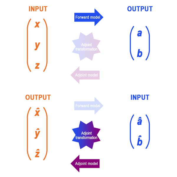
These images show the relationships between forward and adjoint models' inputs and outputs. Adjoint variables are distinguished by their carets (e.g., â).

We want to calculate the sensitivity of J. How much would J change if the forward model's input changes one by one? Here's a way... start with changing x by 1. So, x = 1 | y = 0 | z = 0:

With a=1 and b=4, let's calculate the sensitivity:

That's a lot of steps... is there an easier way? Yes! The "adjoint model", in comparison, allows us to evaluate this sensitivity in one step.

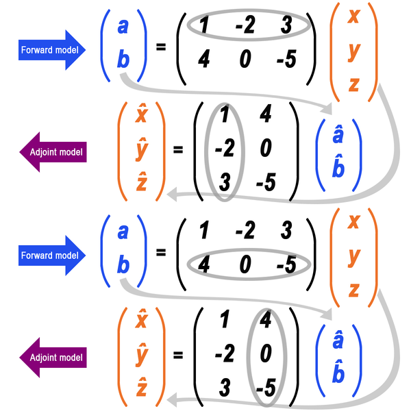
Get ready to enter the "world of the matrix." Remember the equations of the forward model? Each can be shown in matrix form, like this:

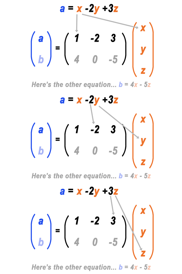
Matrix form makes it easier to show how an adjoint is backward of a forward model. Below, our forward and adjoint models are highlighted. The positions of (a, b) and (x, y, z) are switched for the adjoint variables (â, b̂) and (x̂, ŷ, ẑ). Also, rows in the forward model matrix are columns in the adjoint model matrix.

So, what are the equations for the adjoint model? Click the image below to switch among them.

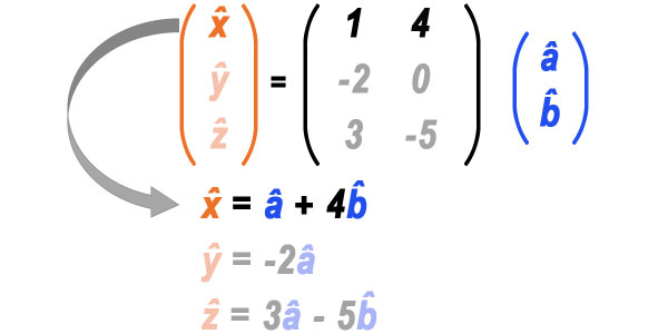
Now that we have the adjoint equations, how do we calculate the sensitivity of J? The adjoint variables are the sensitivity!

Namely, by setting the adjoint model's input (â, b̂) to be the sensitivity of J to (a,b)...

... the adjoint model's output (x̂, ŷ, ẑ) is the sensitivity of J to (x, y, z):

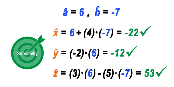
These results match the previous calculations. Happily, this computation requires only one evaluation of the adjoint model instead of the three that were required by the forward model.

These equations are simple and thus the efficiency of using the adjoint might not be obvious. But imagine the model being more complex such as in ECCO, where a single forward model evaluation requires days of computation on a state-of-the-art supercomputer and its input consists of millions of variables! On the other hand, using the adjoint model requires only one evaluation.

Thus, it is impractical to use the forward model to evaluate the sensitivity of a model like ECCO’s, whereas it is routine using its adjoint. This computational efficiency is what makes an adjoint model indispensable.

How is an adjoint used?

Sensitivity (gradient) is foundational in calculus used in every branch of science and engineering that employs math. Just as how calculus has advanced these disciplines, adjoint-derived sensitivities provide new insight into problems.

Adjoint models were first introduced in oceanography in the context of data assimilation. Based on sensitivity of model-data differences, adjoint models are used to fit corresponding forward models to observations. This approach is also at the heart of ECCO's state estimation products. Values of an adjoint's sensitivity also tell us what observations are most effective for monitoring different quantities of interest and are useful in designing observing systems. Check out this StoryMap for one example:

The adjoint also provides an effective means to investigate the workings of the ocean. For instance, a change in passive tracer – think of dye spreading in water – can tell us how that tracer-tagged water moves over time, in other words, the "fate" of the water. In contrast, the sensitivity of such quantity to tracer concentrations in the past is determined using the adjoint. It tells us where that tracer-tagged water came from, or the "origin" of the water.

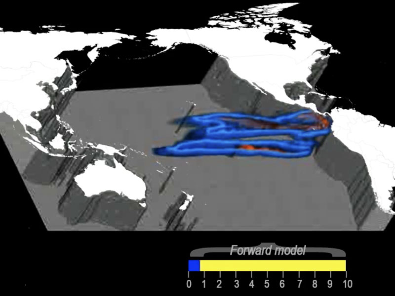
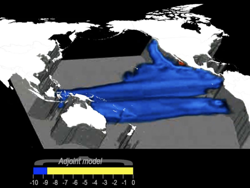
These movies show how ECCO is used to examine the origin and fate of water in the surface layer of the central Equatorial Pacific (5°S-5°N, 150°W-90°W) at a chosen year ("0") deduced by a passive tracer (years > 0) and its adjoint (years < 0). The adjoint passive tracer is evaluated backward in time but below is animated forward in time. The evolving spatial extent of the tracer, shown in blue, illustrates the pathway of ocean circulation. Note the vast spatial extent of both origin and fate compared to where the tracer is at year 0. Click here to watch both movies together.

Adjoint models are also employed in studies of causation and attribution ("adjoint gradient decomposition"). With this method, sensitivity is used to quantify effects of different elements driving the ocean. Thus, it provides a tool to assess the relative contributions of various drivers (e.g., north-south wind, east-west wind). In contrast to common practice of using correlation, which quantifies similarities, adjoints reveal causation thanks to first principles they are based on. Check out these StoryMap examples:

What's special about ECCO's adjoint?

ECCO's ocean model, MITgcm, is one of the few state-of-the-art general circulation models that has an adjoint readily available.

Coding the adjoint of a complex numerical model is time consuming and difficult. It can be comparable in effort to development of the forward code itself. However, ECCO's underlying ocean model was purposefully written to obtain its adjoint code in an automatic way. How? Using Algorithmic Differentiation (AD).

AD software can automatically transform computer programs line by line into their adjoint. In fact, MITgcm was created with automatic differentiation in mind, with ECCO's ocean state estimation advancing hand-in-hand with establishing such tools. As MITgcm was developed, new features were advanced in AD to work seamlessly with ocean circulation models. Furthermore, the style of MITgcm's programming was restricted to those amenable to AD. Today, a rigorous process is still in place to test the "adjointability" of any new feature introduced in MITgcm. This assures availability of the adjoint for the latest version of MITgcm for use in ECCO's ocean state estimation and its various applications.